Data-Driven Control: Achieving Balance in Example Systems

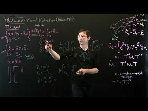
Welcome back! In our previous video, we explored how the dynamics of linear dynamical systems can be transformed using invertible coordinate transformations. By converting the original coordinates (x) into new coordinates (z), we observed that the system’s dynamics also changed, with new parameters (a hat, b hat, and c hat) replacing the original ones (a, b, and c). This transformation also affected the controllability and observability Gramians, which play a crucial role in system analysis and control design.

In this article, we will delve into a simple example to illustrate how these concepts of balancing can be applied. It is important to note that the foundations of balance model reduction stem from a seminal paper by Moore in 1981. Moore’s work laid the groundwork for understanding the existence of transformations that balance the Gramians, both theoretically and with real systems. Our approach is inspired by this pioneering work.

An Example of Balancing

Let’s dive into a straightforward example to demonstrate the process of balancing. Suppose we have a system described by the following differential equations:

d/dt x1 = -1*x1
d/dt x2 = -10*x2

Here, we have intentionally decoupled the system to make it easier to understand. Additionally, let’s assume our state vector x is initially set to [10^-3, 10^3], and our measurement vector y is [10^3, 10^-3]. Notice that x1 is much harder to control than x2, while x1 is significantly easier to measure than x2.

We can perform a simple balancing transformation to address this imbalance. By introducing new coordinates z1 and z2, defined as:

z1 = 10^3 * x1
z2 = 10^-3 * x2

we can rescale x1 to make it a thousand times bigger and rescale x2 to make it a thousand times smaller. In matrix form, this transformation can be represented as:

Z = [10^3  0
      0   10^-3] * X

where Z and X are the new and original state vectors, respectively. The matrix T represents the transformation from X to Z, and its inverse, T inverse, represents the transformation from Z to X.

Balanced Dynamics in the New Coordinates

With this transformation, we can now observe how the dynamics of the system change in the new coordinates, Z. The dynamics of z1 remain unchanged, as the multiplication and division by 10^3 cancel each other out. However, the dynamics of z2 are altered due to the rescaling.

The resulting dynamics in z-coordinates are:

d/dt z1 = -1*z1
d/dt z2 = -10*z2

These dynamics indicate that the system’s inputs and outputs are now balanced, regardless of their initial imbalance. The extreme discrepancy between controllability and observability in the original coordinates is mitigated in the new coordinates, where both states are equally controllable and observable.

This example serves as a simplified illustration of the balancing process. Moore’s original work demonstrated how this technique can be applied to systems of much larger dimensions, such as a thousand by thousand or even a million by million. The goal is to design a transformation matrix, T, that balances the Gramians of the system.

FAQs

Q: What is the significance of balancing a system’s dynamics?
A: Balancing a system’s dynamics is crucial as it enables us to address any imbalances between the controllability and observability of the system’s states. By transforming the coordinates, we can achieve balanced dynamics, making it easier to control and observe the system.

Q: How does balancing impact system analysis and control design?
A: Balancing has a significant impact on system analysis and control design. It allows us to identify the most controllable and observable states, aiding in control system design and optimization. Additionally, it helps in reducing the dimensionality of large-scale systems, making the analysis and control tasks more manageable.

Q: Can balancing be applied to nonlinear systems?
A: The concept of balancing primarily applies to linear systems. However, there have been extensions and adaptations to apply balancing techniques to certain classes of nonlinear systems. These extensions involve linearizing the system around an operating point and then applying the balancing methodology.

Q: How does balancing relate to model reduction?
A: Balancing is closely related to model reduction techniques. By reducing the system’s dimensionality while preserving the essential dynamics, balancing allows for more efficient analysis and control of large-scale systems. Balanced systems provide a simplified representation that retains important system characteristics.

Conclusion

In this article, we explored the concept of balancing in the context of data-driven control systems. By transforming the coordinates and rescaling the states, we achieved balanced dynamics, equalizing the controllability and observability of the system’s states. Although we presented a simplified example, the principles of balancing can be extended to large-scale systems, enabling efficient analysis and control.

For more information on data-driven control and related topics, visit Techal.

Thank you for taking the time to explore the world of data-driven control with us!