Who would have thought that a seemingly complex periodic function could be approximated so beautifully? In this fascinating journey, we will explore the wonders of Fourier series and how it allows us to capture the essence of any periodic continuous function using a combination of sines and cosines of increasing frequencies. Today, we will delve into Python to witness the magic unfold, using a triangular hat function as our example. So fasten your seatbelts and let’s embark on this exciting adventure together!
Contents
Unveiling the Fourier Series
Imagine having an arbitrary function that repeats itself over a specific interval. The Fourier series aims to approximate this periodic function by summing an infinite number of sines and cosines, each with increasingly higher frequencies. How does it work, you may wonder? Well, by gradually adding up these sine and cosine waves, we flawlessly recreate the original periodic function.
Now, let’s get technical. To achieve this approximation, we need to determine the coefficients for each sine and cosine wave. These coefficients, denoted as Ak and Bk, are derived by projecting the function onto the corresponding sine and cosine waves. In simpler terms, we compute the inner product of the function with the sine and cosine waves. This mathematical dance allows us to obtain the coefficients and create a mesmerizing representation of the original function.
Python and the Triangular Hat Function
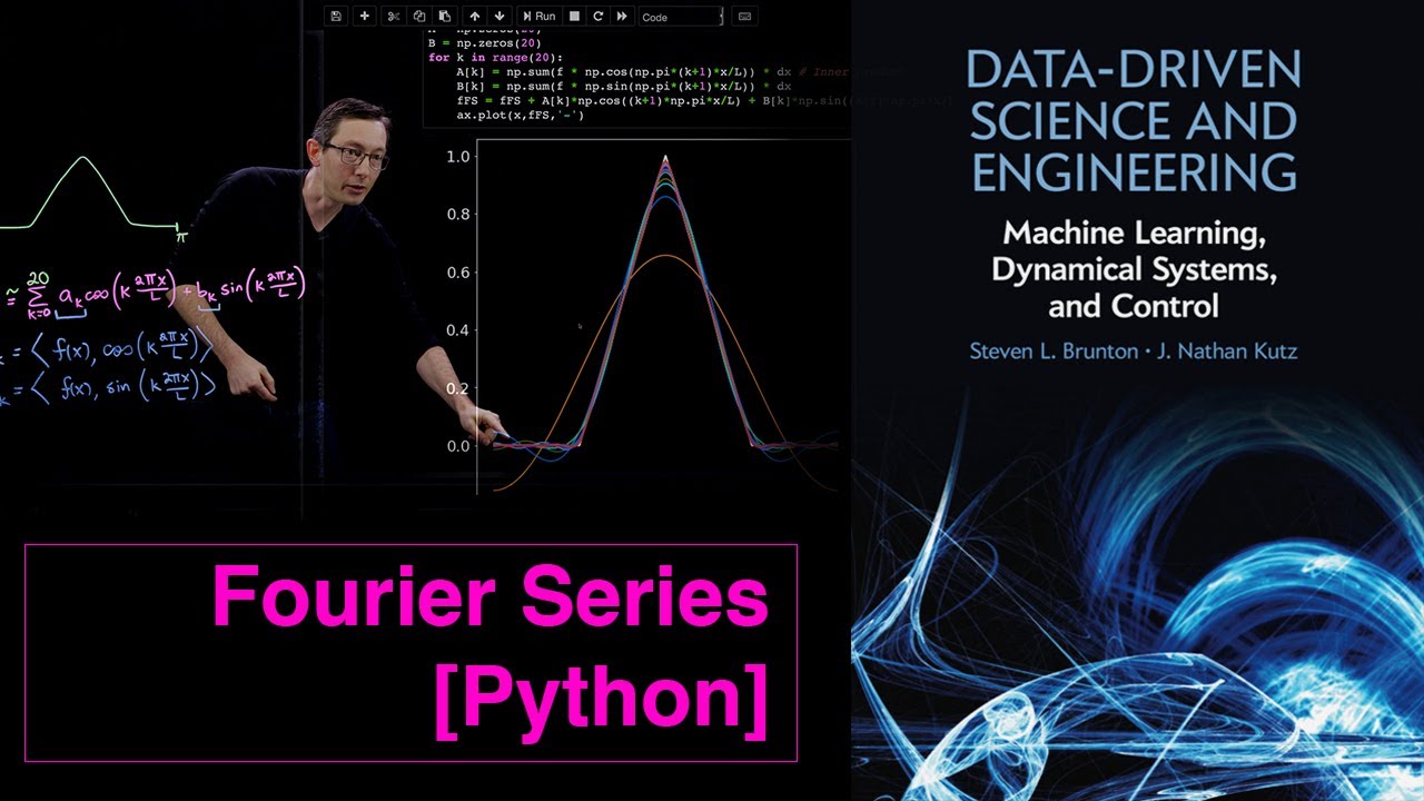
Today, we turn to Python to witness the power of the Fourier series in action. The code provided below, courtesy of the brilliant mind of Daniel Daluz, will guide us through the process. Remember, you can download the code from databookuw.com or access it on GitHub.
# code snippets removed for brevityLet’s break down this Python code and see how it works. First, we define the domain of the function, from -π to π, using a small interval (ΔX) of 0.001 for precise calculations. Then, we define the triangular hat function itself. This unique hat function is crafted by dividing the domain into quarters. The first and last quarters have a value of zero, while the middle second and third quarters generate a positive and negative slope that meet in the middle, creating the distinct triangular shape.
But wait, there’s more! The real magic happens when we compute the Fourier series. In this code snippet, we sum the sines and cosines of different frequencies, ranging from K=0 to K=20. However, note that we don’t actually add an infinite number of terms – we’re only truncating it at a certain value (R) to create a finite approximation. Similar to the singular value decomposition, we approximate the function using a limited number of sine and cosine modes.
Now let’s put it all together. We traverse through K=1 to K=20, calculating the Ak and Bk coefficients by computing the inner products with the given function. These inner products are reminiscent of the familiar integral forms, but adapted for discrete data vectors. To obtain accurate results, we normalize the inner products by the ΔX interval. Finally, we sum the sines and cosines, proportionally weighted by their coefficients, to create the approximated function. The resulting plot showcases the astounding accuracy of this method, as the function aligns closer and closer to the original triangular hat shape with each added term.
The Grand Reveal: Plotting Amplitudes and Reconstruction Error
As if that wasn’t enough, we have yet another treat in store! We can visualize the amplitudes of each cosine term and examine the reconstruction error for different numbers of modes. By plotting the amplitudes and reconstruction error against the number of modes, we unlock even deeper insights into the power of the Fourier series.
In the plots, you’ll notice the x-axis representing the number of modes, ranging from 0 to 100. The y-axis reveals the amplitudes of the cosine terms and the reconstruction error, respectively. As we increase the number of modes, the amplitudes showcase their oscillatory behavior. Interestingly, every fourth mode almost reaches zero, a fascinating consequence of the symmetry embedded in the chosen function.
But here’s the real treasure: the reconstruction error. This graph demonstrates the true essence of the Fourier series approximation. As the number of modes increases, the reconstruction error consistently decreases. This beautiful monotonic decline reveals the power of the asymptotic approximation – the more terms we include, the better the approximation becomes. The error never backtracks; instead, it steadily dwindles as we add more terms to the series. With as few as 20 modes, this method already produces a remarkable approximation.
The Journey Continues
Our adventure with Fourier series has just begun. In future lectures, we will explore potential pitfalls and delve into the discrete Fourier transform, which allows rapid computation of these mesmerizing approximations. So stay tuned for more mind-bending revelations!
In the meantime, if you want to dive deeper into the wonders of technology and gain valuable insights, don’t forget to visit Techal. There you’ll find a treasure trove of knowledge waiting to be explored.
Thank you for joining us on this exhilarating journey into the enchanting realm of Fourier series. Until next time, my curious friends!
