Are you ready to dive into the world of logistic regression? In this article, we will explore the concept of maximum likelihood and how it is used to fit a line in logistic regression models. Get ready to discover the secrets behind the best-fitting squiggles and how they optimize data fitting.

Contents
Unveiling Logistic Regression
Before we delve into maximum likelihood, let’s have a quick recap on linear regression. In linear regression, we fit a line to a given set of data using the least squares method. By measuring the residuals and squaring them, we find the line that minimizes the sum of squared residuals. However, logistic regression takes a different approach.
The Mysterious Transformation
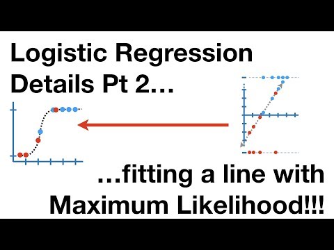
In the realm of logistic regression, we transform the y-axis from the probability of an event to the log odds of that event. This transformation pushes the raw data towards positive and negative infinity, making the use of least squares impossible. In its place, we turn to maximum likelihood.
Unveiling Maximum Likelihood
Maximum likelihood is the key to finding the best-fitting line in logistic regression. To begin, we project the original data points onto a candidate line, giving each sample a candidate log-odds value. This log-odds value is then transformed into a candidate probability using a fancy formula.
This formula, which beautifully reorders the transformation from probability to log odds, involves various mathematical steps. By substituting the log odds values for the candidate points, we obtain the corresponding probabilities. These probabilities give us the y-coordinates on the squiggle.
The Dance of Likelihood
Now that we have our squiggle, it’s time to determine the likelihood of the data given this shape. We start by calculating the likelihood of the obese mice. This likelihood is equal to the y-axis value where the point intersects the squiggle.
For the non-obese mice, the likelihood is calculated as one minus the probability of being obese. The lower the probability of obesity, the higher the probability of not being obese. By including the individual likelihoods of both obese and non-obese mice, we can calculate the overall likelihood.
The Power of Log-Likelihood
While it is possible to calculate the likelihood as the product of individual likelihoods, statisticians prefer to calculate the log of the likelihood, also known as the log-likelihood. Adding the logs of individual likelihoods instead of multiplying them, we obtain the log-likelihood of the data given the squiggle.
The algorithm used to find the line with the maximum likelihood is quite intelligent. It rotates the line in a way that increases the log-likelihood, ultimately finding the optimal fit. After a few rotations, we arrive at a line that maximizes the likelihood, giving us the best fit.
Beyond Fitting Lines
But wait, there’s more to logistic regression than just fitting lines. We also want to determine if the line represents a useful model. For this, we need to calculate an r-squared value and a p-value. However, in logistic regression, we don’t have the luxury of using residuals as in linear regression. Fear not, we will explore these concepts in a future article.
And there you have it! The intriguing world of logistic regression and the power of maximum likelihood. We hope you enjoyed this journey, and if you want to learn more, subscribe to our channel. Don’t forget to support us by liking and sharing. Until next time, keep questing!