In the world of applied mathematics, ordinary differential equations (ODEs) play a vital role in describing how quantities change over time. Whether it’s the growth of a population, the stock market, or even the spread of a virus, ODEs allow us to understand and simulate complex systems. In this article, we’ll focus on numerical methods for integrating ODEs, specifically the forward Euler method.
Contents
Understanding ODEs
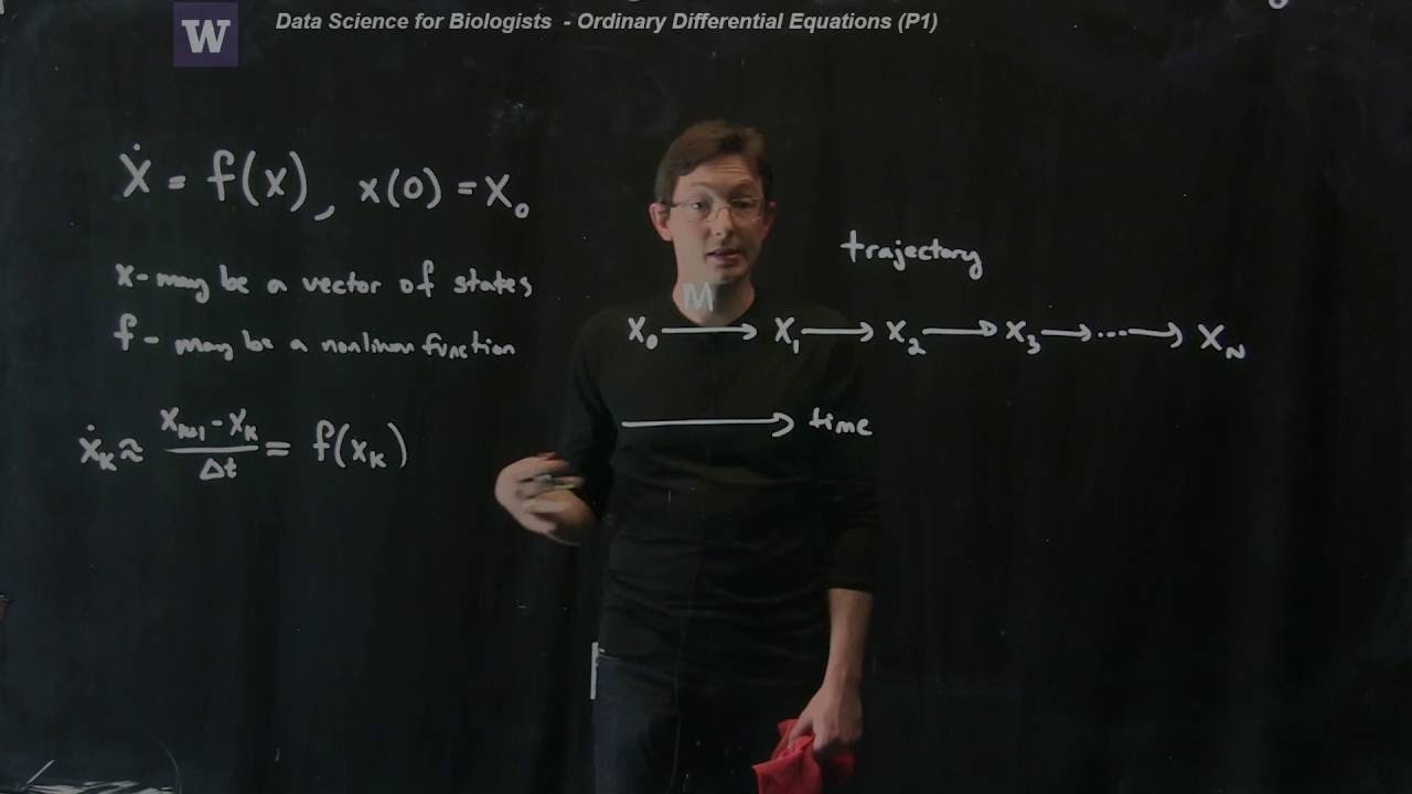
An ordinary differential equation is typically written as:
x' = f(x)Here, x represents a vector of states, and f is a nonlinear function that describes how these states change over time. Consider a population dynamics example, where x represents the number of bunnies and the number of wolves at a given time. The population of bunnies depends on the number of wolves and vice versa. This interaction forms a resource-constrained population problem.
To approximate the solution of an ODE, we need to discretize the system. This means stepping the system forward in time on a computer and simulating the outcome. The goal is to build a trajectory, a sequence of states that represent the system’s behavior over time.
The Forward Euler Method
To approximate the derivative x', we can use finite difference approximations. The forward difference method approximates the derivative at time k by considering the change in x from time k to k + 1:
x_k+1 = x_k + Δt * f(x_k)Here, Δt represents the time step, and f(x_k) is the value of the function f at time k. Starting with an initial state x_0, we can iteratively compute x_1, x_2, and so on. This approach is known as the forward Euler method.
While the forward Euler method is straightforward and easy to implement, it comes with limitations. It assumes a constant rate of change over each time step, which may not be accurate for complex systems. As a result, it may not provide the most precise results. However, the simplicity and efficiency of the method make it a popular choice for many applications.
Comparing Forward and Backward Euler Methods
The forward Euler method is just one of many numerical methods for integrating ODEs. Another common approach is the backward Euler method, also known as the implicit Euler method. Unlike the forward Euler method, the backward Euler method considers the change in x from time k to k + 1:
x_k+1 = x_k + Δt * f(x_k+1)Here, the value of f at time k + 1 is used, making it an implicit function of x_k+1. This implicit nature of the backward Euler method can make it more accurate and stable than the forward Euler method. However, it also requires solving for x_k+1, which can be challenging in some cases.
Choosing between the forward and backward Euler methods depends on the specific problem at hand. While the backward Euler method offers improved accuracy and stability, its implicit nature can make it more computationally demanding.
Applying the Forward Euler Method to Population Modeling
Let’s consider a specific example: a population model. Suppose we have a population of bunnies and wolves, where the growth of each population depends on the other. We can write the ODEs for this model as follows:
b' = f(b, w)
w' = g(b, w)
Here, b represents the number of bunnies, w represents the number of wolves, and f and g are nonlinear functions that describe how the populations change over time.
By applying the forward Euler method, we can approximate the solution of these ODEs step by step, iteratively updating the populations at each time step. This approach allows us to simulate the dynamics of the population model over time, gaining valuable insights into the interplay between bunnies and wolves.
Q: What is an ordinary differential equation (ODE)?
A: An ordinary differential equation describes how quantities change over time. It consists of a function that relates the derivative of a variable to the variable itself.
Q: What is the forward Euler method?
A: The forward Euler method is a numerical method for integrating ODEs. It approximates the derivative of a variable at each time step by considering the change in the variable over that time step.
Q: What is the backward Euler method?
A: The backward Euler method is an alternative numerical method for integrating ODEs. It approximates the derivative of a variable by considering the change in the variable from one time step to the next, using the value of the function at the next time step.
Numerical methods, such as the forward Euler method, allow us to approximate solutions for ordinary differential equations. By discretizing the system and stepping it forward in time, we can simulate the behavior of complex systems accurately. While the forward Euler method is simple and efficient, other methods, like the backward Euler method, offer improved accuracy at the cost of increased computational complexity.
Understanding and applying numerical methods for integrating ODEs is essential in various fields, including mathematics, physics, engineering, and biology. By leveraging these methods, we can gain valuable insights into the behavior and dynamics of real-world systems.
To explore more about the world of technology and its cutting-edge advancements, visit Techal.
