Welcome to the enthralling world of Long Short-Term Memory (LSTM) with PyTorch + Lightning. Get ready for an extraordinary journey where complexities transform into simplicities and miracles become everyday occurrences. This is not just an ordinary tutorial, but a captivating adventure that will make your coding life a breeze.
Contents
Unveiling the Secrets of LSTM
Before we dive into the depths of LSTM, let’s take a quick detour to understand its fundamentals. LSTM is a powerful algorithmic technique used to process and make predictions based on sequential data. In our case, we’ll be examining sequential stock market data for two companies, Company A and Company B.
Imagine the stock values for both companies plotted on a graph, with the y-axis representing the stock value and the x-axis representing the day the value was recorded. Surprisingly, we observe that the only notable variations occur on day one and day five. On day one, Company A’s value is at zero while Company B’s value is at one. Then, on day five, Company A returns to zero and Company B returns to one. However, on all the other days (Days 2, 3, and 4), both companies have the exact same stock values.
In order to predict the stock values on day five accurately, we need an LSTM model that can remember what happened on day one. This involves running the sequential data from Days 1 through 4 through an unrolled LSTM. By doing so, we can predict the values for day five for both companies.
The Magic of PyTorch + Lightning
Now that we comprehend the underlying concept of LSTM, let’s proceed to implement it using the powerful combination of PyTorch and Lightning. We will code the LSTM unit from scratch, creating and initializing all the weight and bias tensors needed for the implementation.
First, we import the PyTorch library, which allows us to create and manipulate tensors to store numerical values, including raw data and weights. Additionally, we import torch.nn to incorporate the weight and bias tensors into the neural network.
Our next step is to define the LSTM unit. We start with the initialization method, where we create and initialize the weight and bias tensors for the LSTM unit using a normal distribution. This ensures randomness in the initialization process. Then, we move on to coding the main LSTM unit, which consists of three stages:
-
Stage 1: Determining the percentage of long-term memory to remember: We calculate the percentage of long-term memory to remember by combining the short-term memory and input values with their corresponding weights and a bias. The result is passed through a sigmoid activation function.
-
Stage 2: Creating a potential long-term memory: We calculate the percentage of the potential long-term memory to remember by combining the short-term memory and input values with their corresponding weights and a bias. The result is passed through a sigmoid activation function. Next, we calculate the potential long-term memory by passing the result through a tanh activation function.
-
Stage 3: Creating a new short-term memory: We determine the percentage of the new short-term memory to remember by combining the updated long-term memory with the short-term memory and passing it through a sigmoid activation function. Finally, we return the updated long-term and short-term memories.
With the LSTM unit implemented, we can now create the forward method, which makes a forward pass through the unrolled LSTM unit. This method takes an array containing the stock market values for days one through four for one of the companies. We initialize the long-term and short-term memories to zero and then pass the values through the LSTM unit, updating the memories at each step. Finally, we return the final short-term memory as the output.
To optimize the weights and biases, we use the Adam optimizer, which is similar to stochastic gradient descent but tends to converge faster. We configure the optimizer by setting the learning rate to 0.1.
The next step is the training process. We create a LightningTrainer object and set it to train for a maximum of 300 epochs. We then call the fit method to train the LSTM model with the training data, using the optimized weights and biases. After training, we print the predictions for both companies, which should be significantly improved.
To visualize the training progress, we use TensorBoard, a powerful tool that allows us to generate insightful graphs from the log files. By analyzing the loss values and the predictions for each company, we can assess the effectiveness of our training and determine if more training is necessary. In this case, it seems that more training would lead to even better predictions.
From Scratch to Simplicity: The Power of nn.LSTM
Now that we have seen the process of creating an LSTM from scratch, it’s time to explore the simplicity of using PyTorch’s nn.LSTM function. By taking advantage of this function, we can streamline the code and achieve the same results with less effort.
We create a new class called LightningLSTM, which inherits from the LightningModule class. The initialization method is straightforward, as we only need to call nn.LSTM to create the LSTM unit.
In the forward method, we transpose the input data to match the shape expected by nn.LSTM. We then pass the transposed data through the LSTM unit and extract the prediction from the last LSTM unit, which corresponds to the prediction for day five. Finally, we return the prediction.
The configure_optimizers method remains the same, but we increase the learning rate to 0.1 to demonstrate the faster convergence of the Adam optimizer.
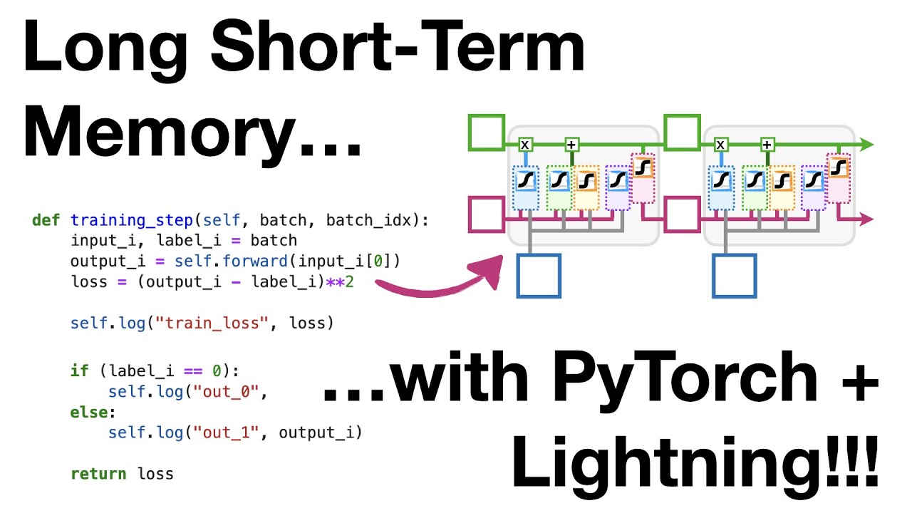
The training step method is identical to the previous implementation, calculating the loss and logging the progress.
With the LightningLSTM class ready, we can now create the model and print the predictions. As before, we realize that the initial predictions are not satisfactory, so we proceed with the training process.
We create a new LightningTrainer object, this time limiting the training to 300 epochs due to the higher learning rate. By updating the log files every two steps, we can generate more frequent and comprehensive graphs using TensorBoard.
After training, we print the updated predictions, which should show significant improvement. We can also analyze the graphs in TensorBoard, which indicate that further training is unnecessary as the curves have flattened out.
Conclusion
Congratulations on completing this adventure into the realm of LSTM with PyTorch + Lightning! You have discovered the power of sequential data analysis and learned how to implement LSTM from scratch or with the help of PyTorch’s nn.LSTM function.
If you want to delve deeper into statistics and machine learning, be sure to check out the StackQuest PDF study guides and the book “The StatQuest Illustrated Guide to Machine Learning,” available at Techal.org. And if you enjoyed this article, please consider supporting StackQuest through Patreon, becoming a channel member, or purchasing original songs or merchandise. Your support is greatly appreciated!
Until the next thrilling StatQuest, happy coding!
