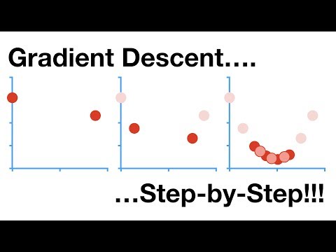
Welcome to Techal! In this guide, we will explore the powerful algorithm known as Gradient Descent, step by step. Whether you’re into statistics, machine learning, or data science, understanding Gradient Descent will give you a strategic advantage in optimizing various optimization problems.

Contents
Introduction
In the vast field of data science, optimization is a recurring theme. We often encounter scenarios where we need to find the best values for parameters such as intercepts, slopes, or clustering. This is where Gradient Descent comes into play. This algorithm is incredibly versatile and can optimize a wide range of problems.
Fitting a Line with Gradient Descent
To illustrate how Gradient Descent works, let’s start with a simple example. Imagine we have a dataset with weight values on the x-axis and corresponding height values on the y-axis. We want to fit a line to this data by finding the optimal values for the intercept and slope.
To begin, we pick a random value for the intercept as an initial guess. Let’s say we start with 0. We then evaluate how well this line fits the data using the sum of the squared residuals as a measure of fit. The goal is to minimize this value.
To calculate the sum of the squared residuals, we compare the observed height with the predicted height for each data point. The predicted height is obtained by plugging the weight value into the equation for the line. By summing the squared differences between the observed and predicted heights, we obtain the sum of the squared residuals.
Finding the Optimal Intercept
Now, let’s use Gradient Descent to find the optimal value for the intercept. We start with our initial guess of 0 and calculate the sum of the squared residuals. Next, we take the derivative of the sum of the squared residuals with respect to the intercept. This derivative represents the slope of the curve at the current intercept value.
Gradient Descent works by taking steps towards the minimum. When the slope is large, we take big steps; when it’s close to zero, we take smaller steps. The step size is determined by multiplying the slope by a learning rate, which controls the size of the steps.
By subtracting the step size from the current intercept, we obtain a new intercept value. We repeat this process, recalculating the sum of squared residuals, derivative, step size, and intercept, until the step size becomes very small or we reach a maximum number of steps.
Through this iterative process, Gradient Descent gradually converges to the optimal intercept value that minimizes the sum of squared residuals. In our example, the optimal intercept is found to be 0.95, matching the least squares estimate.
Estimating Intercept and Slope Simultaneously
Now, imagine we want to estimate both the intercept and the slope simultaneously. We can still use Gradient Descent by taking the derivative of the sum of squared residuals with respect to both parameters.
Similar to the previous example, we start with random values for the intercept and slope. We calculate the sum of squared residuals, take the derivatives, determine the step sizes, and update the intercept and slope accordingly. This process continues until the step sizes become very small or we reach the maximum number of steps.
By following these steps, we can find the optimal values for both the intercept and the slope, giving us the best fitting line for the data. As before, the sum of squared residuals serves as the loss function that we aim to minimize.
FAQs
Q: Can Gradient Descent optimize multiple parameters?
A: Yes, Gradient Descent can optimize multiple parameters. By taking the derivatives of the loss function with respect to each parameter, we can iteratively update their values until convergence is achieved.
Q: What if there are millions of data points? Won’t the calculations take a long time?
A: Yes, calculating the derivatives can be time-consuming when dealing with a large amount of data. In such cases, Stochastic Gradient Descent can be used, which randomly selects a subset of the data at each step, reducing the computational burden.
Q: How does Gradient Descent know when to stop taking steps?
A: Gradient Descent stops iterating when the step size becomes very small, indicating that it has reached a near-optimal solution. Additionally, there is often a limit on the maximum number of steps, ensuring that the algorithm doesn’t run indefinitely.
Conclusion
Gradient Descent is a powerful algorithm that allows us to optimize parameters in various optimization problems. By iteratively updating parameter values based on derivatives and step sizes, it guides us toward the optimal solution. Whether it’s fitting lines, clustering, or solving complex optimization problems, Gradient Descent is a valuable tool in the field of data science.
We hope this guide has shed light on Gradient Descent and its step-by-step process. If you want to delve deeper into the world of technology, stay tuned to Techal, your ultimate source for insightful analysis and comprehensive guides.
Techal – Empowering your knowledge in the ever-evolving world of technology.


