Have you ever wondered how we can break down complex functions into simpler waves? Enter the Fourier Transform, a powerful mathematical tool that allows us to analyze any function in terms of its underlying frequencies. In this article, we will delve deeper into the world of Discrete Fourier Transforms (DFTs) and explore how they work. So, hold on tight and get ready to unravel the secrets of frequency analysis.
Contents
Introduction: Unlocking the Power of Discrete Fourier Transforms
Last time, we briefly touched on the concept of Discrete Fourier Transforms. These transforms take data points sampled from a function and convert them into coefficients of sine and cosine waves. These coefficients represent the amplitudes of the different frequencies needed to perfectly reconstruct the original function. While the math behind DFTs can seem a bit complex, the basic idea is simple and intuitive.
Understanding the nth Frequency and the DFT Matrix
To fully grasp the power of DFTs, let’s introduce the concept of the nth frequency, denoted as Omega n. This frequency can be represented as a complex number, comprising both cosine and sine components. By adding up sine and cosine waves of higher and higher frequencies, we can reconstruct the original function.
To transform our data into Fourier coefficients, we need a matrix. This matrix, known as the Discrete Fourier Transform (DFT) Matrix, serves as our key to unlock the world of Fourier analysis. The DFT Matrix allows us to multiply our data vector by this matrix and obtain the desired coefficients.
The Mysteries of the DFT Matrix
The DFT Matrix is a fascinating construct. It consists of a pattern of increasing powers of Omega n, with each element representing a specific frequency component. The first row and column of the matrix are entirely composed of ones, while the subsequent elements follow the pattern of Omega n raised to various powers.
This powerful matrix, when multiplied by our data vector, produces the Fourier coefficients we seek. These coefficients hold significant physical meaning, as they represent the amplitudes of the different frequency components necessary to reconstruct our data perfectly.

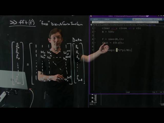
Unleashing the Power of the DFT Matrix with MATLAB
Now that we understand the DFT Matrix, let’s dive into the practical side of things. We can leverage MATLAB’s built-in Fast Fourier Transform (FFT) command to obtain Fourier coefficients with ease.
By simply using the fft command in MATLAB, we can compute the Fourier coefficients of our data vector. This command performs the same operation as multiplying our data by the DFT Matrix, but with enhanced speed and efficiency. Comparing the results obtained from MATLAB’s FFT command and the manual matrix multiplication shows that they are identical, confirming the validity of the FFT command.
Exploring the Visualization of the DFT Matrix
To add a visual element to our exploration, let’s take a peek into the visual representation of the DFT Matrix. With MATLAB’s image command, we can generate a scaled image of the real part of the DFT Matrix. This visualization showcases the intricate patterns and multiscale features inherent in the matrix.
Experimenting with different screen resolutions yields interesting rendering effects, revealing the different patterns that emerge. It’s fascinating to observe how the DFT Matrix reacts to various resolutions, and we encourage you to explore this phenomenon on your own computer.
FAQs
Q: What is the purpose of the DFT Matrix?
The DFT Matrix allows us to convert our data vector into Fourier coefficients, representing the amplitudes of the different frequency components needed to reconstruct the original function accurately.
Q: How does MATLAB’s FFT command compare to manual matrix multiplication?
MATLAB’s FFT command performs the same calculation as manual matrix multiplication, but with enhanced speed and efficiency. The results obtained from both methods are identical, validating the accuracy of the FFT command.
Q: Can the DFT Matrix be computed faster using vectorized methods?
Yes, nested for loops are computationally expensive in MATLAB. Leveraging vectorized computations, such as by using the meshgrid function, significantly improves the speed of the DFT Matrix calculation.
Conclusion
In this article, we’ve explored the intriguing world of Discrete Fourier Transforms (DFTs). By understanding the concept of frequencies and harnessing the power of the DFT Matrix, we can analyze complex functions in terms of their underlying components. MATLAB’s FFT command provides a fast and efficient way to compute Fourier coefficients, empowering us to unleash the full potential of frequency analysis.
So, the next time you encounter a complex function, remember the insights gained from our exploration of DFTs. With the help of the DFT Matrix and MATLAB’s FFT command, you’ll be well-equipped to dissect and understand the underlying frequencies that shape the world of technology.
Learn more about the power of frequency analysis and explore further technology topics on Techal. Happy analyzing!
